Portfolio Backtest
Portfolio Backtest replays one or more portfolio configurations on historical data. It combines allocations, strategies, cash flows, rebalancing rules, and optional tax-aware accounting in one analysis.
Open Portfolio Backtest →Use this when
Use Portfolio Backtest to ask "what would this portfolio have done over this exact stretch of history?" Pick an allocation, pick dates, and read the resulting equity curve, drawdowns, and metric table.
Good for
- Comparing two or three portfolios on the same window.
- Seeing how rebalancing rules, cashflows, or glidepaths shape outcomes.
- Inspecting tax drag for a taxable account with explicit lots.
Reach for a different tool when
- Probability ranges or failure rates. Use Monte Carlo instead.
- Searching for an optimal weight set. Use Portfolio Optimizer instead.
Portfolio Backtest walkthrough
Start with one portfolio and a clear historical window.
Confirm price mode, rebalancing, cashflows, and tax-aware settings before running.
Read the equity curve, drawdown, and metric table together. A different assumption set is a different experiment.
First run
Set the allocation
Use 80% SPY and 20% AGG for the first run.
Use Total return
Total return (adjusted prices) includes dividends and distributions in the return series.
Pick a long window
Use a date range with more than one market regime.
Run and compare
Review value, drawdown, and risk-adjusted metrics before changing inputs.
Video walkthrough
Walkthrough
Video walkthrough
Configuration Guide
Treat these fields as modeling assumptions. Change one at a time when you want to understand what drives a result.
Set the dollar scale and price mode
The first scenario row anchors how every dollar figure in the result is interpreted.
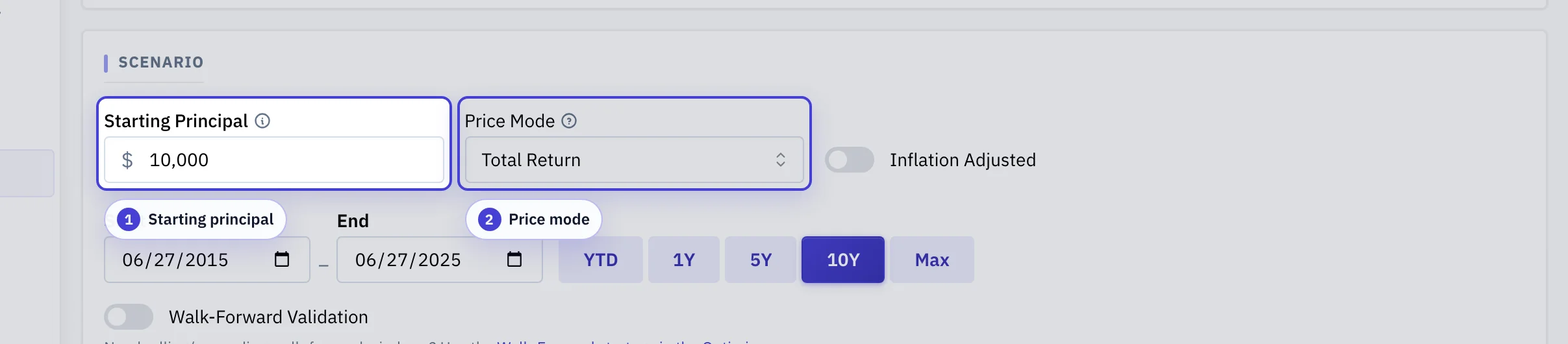
Starting principal: The dollar amount at the start of the backtest. Drives the scale of value, drawdown, and cashflow charts.
Price mode: Total return (adjusted prices) includes dividends and distributions; Raw keeps them separate. Pick Raw only if you also want explicit dividend accounting.
Choose the historical window
The window selects which market regimes the result is sampled from.
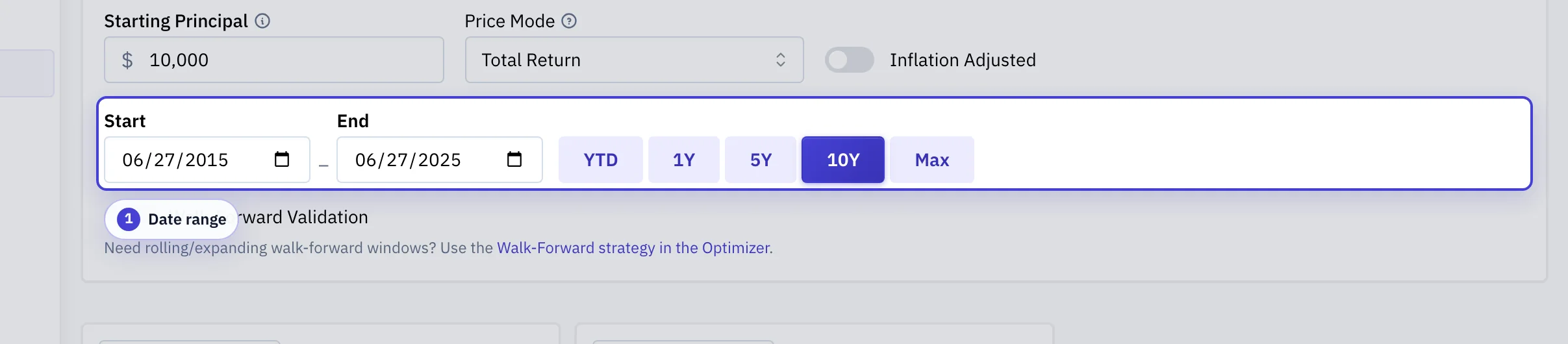
Date range: Pick start and end dates, or use the Max preset to span the full overlap of the included tickers.
Define the portfolio hypothesis
Weights, strategies, and rebalance rules together define what is being tested.
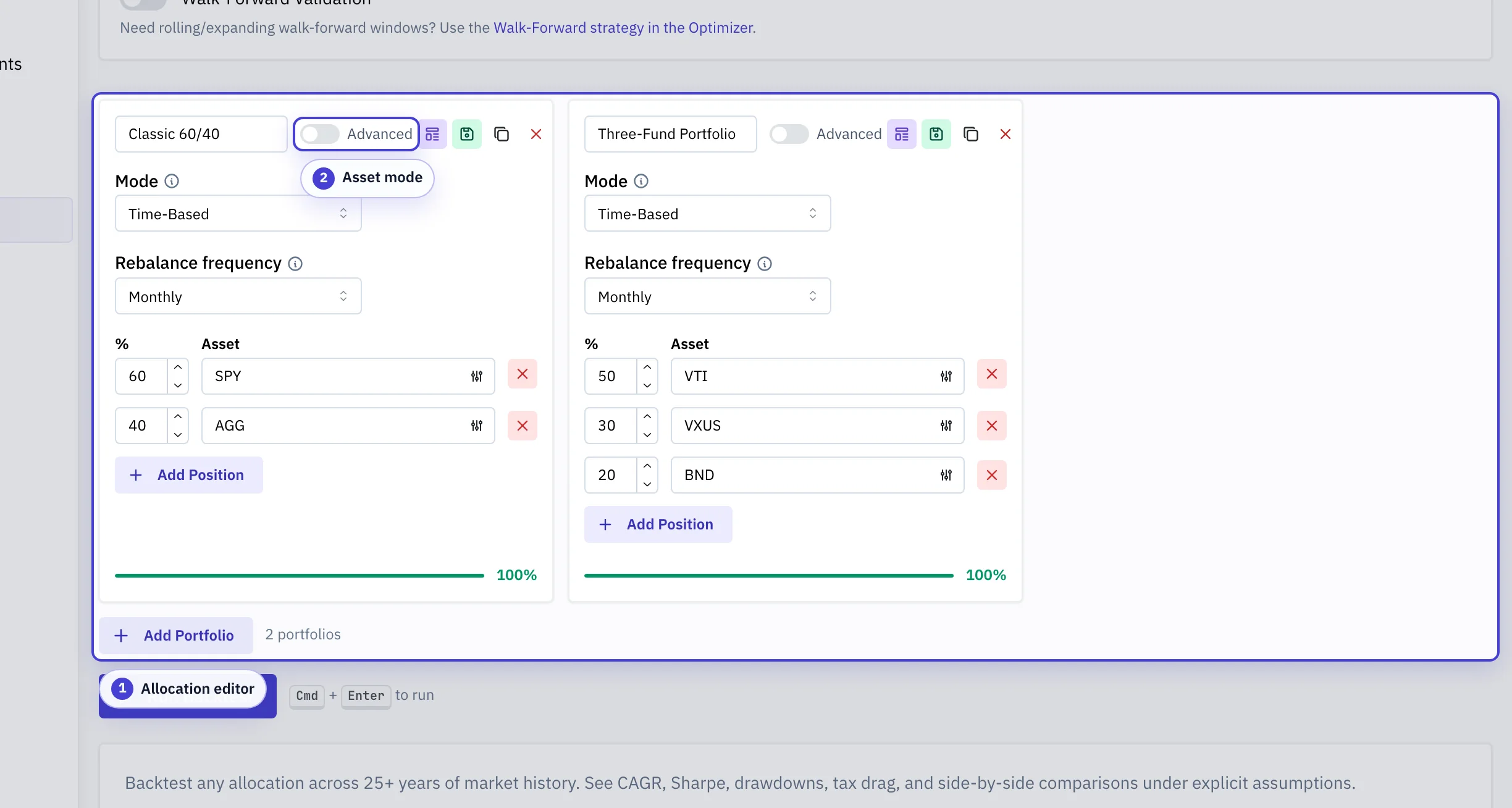
Allocation editor: Add allocations, set weights, link strategies, and pick portfolio-level rebalance rules.
Asset mode: Switch between simple ticker baskets and more elaborate strategies (rules, signals, glidepaths).
| Configuration | What It Means | Why It Matters |
|---|---|---|
| Portfolio allocations | The target asset mix or strategy definition being replayed. | This is the portfolio hypothesis. Changing weights changes both expected return exposure and drawdown behavior. |
| Date range | The historical window used for prices, returns, and events. | A short window can make a strategy look better or worse because it samples only one market regime. |
| Price mode | Total return (adjusted prices) includes dividends and distributions; Raw keeps them separate for dividend accounting. | Use Total return for return comparisons. Use Raw only when you need explicit dividend tracking. |
| Initial value and cashflows | Starting capital plus any recurring or one-time additions and withdrawals. | Cashflows make results path-dependent because deposits and withdrawals happen at specific market levels. |
| Rebalancing | The rule that decides when holdings are traded back toward target weights. | More frequent rebalancing can reduce drift, but it can increase turnover, taxes, and implementation cost. |
| Benchmark | The reference series used for comparison metrics. | Benchmark choice changes relative metrics such as alpha, beta, tracking error, and up/down capture. |
| Tax-aware mode | Adds account type, filing status, income, state, lot selection, and loss assumptions. | After-tax results are not comparable to pre-tax results unless the tax profile is explicit. |
Common pitfalls
Picking too short a date range
A 2015-2020 backtest only saw a single bull regime. Span at least one major drawdown when you can.
Mixing Raw prices with dividend tracking off
Raw keeps dividends and distributions separate, so returns read low. Choose Total return unless you specifically want to inspect dividends.
Comparing a pre-tax run to an after-tax run
Tax-aware mode adds drag and lot-level events. Either run both portfolios with tax-aware on, or both with it off.
Treating one path as predictive
A single historical replay is one sample. For probability ranges, run the same plan in Monte Carlo.
What you'll see in the result
- Equity curve: Cumulative portfolio value through time. The shape, not the endpoint, tells you about drawdowns and recoveries.
- Drawdown chart: Peak-to-trough loss path. Watch the depth and the time-to-recover.
- Metric table: Summary statistics including CAGR, volatility, Sharpe, max drawdown, and benchmark-relative metrics when a benchmark is set.
- Allocation and trading views: Show how the portfolio actually moved through time. Useful for diagnosing whether rebalancing or signals fired as you expected.
- Tax diagnostics: Only present in tax-aware mode. Surfaces total drag, drivers, and warnings instead of a raw lot dump.
Features
- Glidepath portfolios with time-based allocation shifts
- Dividend tracking with configurable reinvestment
- Tax-lot accounting with FIFO, LIFO, HIFO, or optimized selection
- Cash flow schedules (recurring and one-time contributions and withdrawals)
- Regression analysis against any benchmark (alpha, beta, R², tracking error)
- Tax diagnostics for tax-aware runs, including drag drivers, high-impact events, and implementation risks
- Side-by-side comparison of multiple portfolio configurations
- In-sample / out-of-sample holdout split with per-slice metric tables
When To Use It
Use this tool when the question is about how a portfolio configuration would have behaved over a historical window. The result includes the full time series, summary metrics, and supporting tables for that analysis.
For distributional outcomes and failure-rate analysis across many simulated paths, use Monte Carlo instead. See Historical Backtest vs Monte Carlo below for a comparison.
Portfolio Model
| Level | What It Stores | Where It Rebalances |
|---|---|---|
| Portfolio | One or more allocations, portfolio-level cash flows, and portfolio-level rebalancing settings. | Between allocations when portfolio rebalancing is enabled. |
| Allocation | One strategy and its target portfolio weight. | Inside the strategy when the strategy itself holds multiple positions. |
| Strategy | Conditions, positions, signals, and strategy-level rebalance rules. | Within the active condition. |
Main Inputs
- Starting principal: initial portfolio value.
- Date range: historical sample used in the run.
- Price mode: total-return or raw-price return construction.
- Allocations and strategies: the holdings and rules being tested.
- Portfolio rebalancing: how the top-level allocation split is maintained.
- Cashflows: recurring or one-time contributions and withdrawals.
- In-sample / out-of-sample holdout: optional split date used to show separate metrics for the in-sample window and the later out-of-sample window of the same realized run.
Editing A Portfolio
- Add or remove allocations at the portfolio level.
- Edit each allocation's weight and linked strategy.
- Open the strategy editor to add positions, signals, conditions, and strategy-level rebalancing.
- Load a Library strategy or Library portfolio when you need to reuse an existing building block.
See Strategy Leaderboard and Signals for the reusable rule and indicator model used inside the editor.
Rebalancing
Portfolio Backtest has two separate rebalance layers:
- Strategy-level rebalancing: restores weights within the active positions of a strategy.
- Portfolio-level rebalancing: restores the top-level split between allocations.
Both layers can use time-based or threshold-based policies. See the Rebalancing guide for the detailed mode descriptions.
Glidepath Portfolios
A glidepath portfolio changes its target allocation over time. This models the common practice of shifting from growth-oriented to income-oriented holdings as the investment horizon shortens (for example, a target-date retirement fund).
- Static vs glidepath: toggle glidepath mode in the Advanced editor when a portfolio has two or more allocations.
- Milestones: each milestone specifies a date and the target weight for every allocation. The engine uses stepwise resolution: the most recent milestone on or before the current date determines the target weights.
- Dates must be strictly increasing. The milestone weights for each date must sum to 100%.
- Initial allocation rule: if the first milestone falls after the backtest start, the initial sleeve weights from the portfolio editor are used until that milestone takes effect. If a milestone is on or before the start date, its weights override the initial allocation.
Example: a portfolio with two allocations (SPY, AGG) and two milestones shifts from 80/20 on 2010-01-01 to 40/60 on 2020-01-01. In a 2005-2025 backtest the initial weights would be 80/20 (first milestone applies from 2010), then 40/60 from 2020 onward.
Cashflows
- Recurring cash flows: scheduled contributions or withdrawals.
- One-time cash flows: dated events applied once inside the backtest window.
- Sign convention: positive values contribute capital and negative values withdraw capital.
The Cashflows tab in the results section shows each contribution and withdrawal event with dates, amounts, and a running total chart.
In-Sample / Out-Of-Sample Holdout
Portfolio Backtest supports an in-sample / out-of-sample holdout overlay. Choose an in-sample end date, run the backtest, and the results include separate metric tables for the in-sample window and the later out-of-sample window for each portfolio.
- The split uses the realized backtest path. It does not change trades, cashflows, tax-lot events, or rebalancing decisions.
- The requested date snaps to the nearest trading day on or before the selected date. Both sides need enough trading history; otherwise the result shows a warning instead of partial metrics.
- Metric tables use the same metric catalog as the full-period result. Tax-aware and dividend-income metrics are not replayed per slice and are shown as unavailable with a warning.
Tax Diagnostics
When tax-aware mode is enabled, the Tax Diagnostics tab becomes the default tax surface. It summarizes total drag, current-year tax drivers, estimated embedded liquidation drag, high-impact trades, concentrated unrealized gains, and assumptions or confidence flags.
This is the fastest way to answer why a strategy is tax-inefficient before drilling into raw trade logs, lot rows, or wash-sale chains.
Dividend Income
The Dividend Income tab shows annual dividend income as a bar chart, per-portfolio summary metrics (total income, qualified vs ordinary breakdown, payout count), and a sortable table of individual dividend events (ex-date, ticker, shares, per-share amount, income, qualified/ordinary type).
Dividend tracking requires the Raw price mode. Total return (adjusted prices) already bakes dividends into the price series, so using it with dividend tracking would double-count income.
The annual breakdown classifies each dividend as qualified or ordinary. Qualified dividends are taxed at preferential long-term capital gains rates, while ordinary dividends are taxed as regular income.
Rolling Metrics
The Rolling Metrics tab shows windowed calculations for CAGR, volatility, Sharpe, Sortino, and other risk metrics over time. This reveals whether full-period averages mask regime changes. A portfolio with a stable 10% CAGR may have experienced stretches of 20% gains and 5% losses.
The window length is configurable. Shorter windows capture more variation but are noisier; longer windows smooth the series but may obscure transitions.
Risk vs Return
The Risk vs Return tab plots a scatter chart of annualized return against annualized volatility for each portfolio. Point annotations show Sharpe ratio and max drawdown, making it easy to compare risk-adjusted performance when running multiple portfolios.
Seasonality
The Seasonality tab shows average monthly return by calendar month. This can help identify seasonal patterns in portfolio returns. Note that sample sizes per month are small, so patterns may not be statistically significant over shorter backtest windows.
Correlations
The Correlations tab displays a pairwise daily return correlation heatmap. This requires two or more portfolios or a benchmark and is based on daily returns over the backtest window.
Relative Analysis
The Relative Analysis tab shows the performance ratio of each portfolio relative to a baseline (portfolio value divided by baseline value over time). Relative metrics include tracking error, information ratio, and up/down capture ratios. This requires two or more portfolios.
Lump Sum vs DCA
The Lump Sum vs DCA tab runs a separate dollar-cost averaging simulation using the same portfolio configuration. You can configure the DCA frequency (weekly or monthly), deployment duration, and cash yield during the deployment phase.
This compares full immediate deployment against phased entry. The result is path-dependent on the specific historical window. Lump sum wins on average but DCA reduces timing risk.
Allocations
The Allocations tab shows a pie chart grid of target allocation weights for each portfolio, derived from the strategy positions and allocation weights you configured.
Tax-Aware Engine
Tax-aware engine runs the same portfolio settings through a lot-level tax engine. The tax profile controls filing status, income, state, account type, lot selection, and optional loss-harvesting settings. In addition to the raw ledgers, tax-aware runs also produce a canonical diagnostics layer for drag attribution, high-impact events, concentrated-gain warnings, and explicit applicability states.
See Tax-Aware Backtesting for the accounting assumptions and output interpretation.
Ticker Modifiers
Positions can use ticker modifiers when the backtest should use a transformed series rather than the base ticker.
Regression Analysis
The Regression tab runs an OLS regression of each non-benchmark portfolio's returns against the benchmark's returns. It provides a full set of diagnostics for evaluating how much of a portfolio's behavior is explained by benchmark exposure.
- Alpha: the intercept of the OLS regression, representing return generated beyond what beta exposure explains. Reported as both a per-period value and an annualized value.
- Beta: the slope coefficient measuring the portfolio's sensitivity to the benchmark. A beta of 1.0 means the portfolio moves in lockstep with the benchmark; higher values indicate amplified sensitivity.
- R-Squared: the fraction of portfolio return variance explained by the benchmark. Values closer to 1.0 indicate that the benchmark is a strong explanatory factor.
- Correlation: the Pearson correlation coefficient between portfolio and benchmark returns.
- Tracking error: the annualized standard deviation of the return difference between the portfolio and the benchmark. Lower values mean the portfolio tracks the benchmark more closely.
- Information ratio: the annualized excess return divided by the tracking error. A higher value indicates better risk-adjusted outperformance.
Select daily or monthly frequency to change the return interval used in the regression. Monthly aggregation uses geometric compounding of daily returns. The scatter plot shows the fitted regression line; the residual chart surfaces deviations from the linear model.
Compare A Portfolio Against A Benchmark
- Open Portfolio Backtest.
- Configure your portfolio with the target allocations and strategies.
- In the benchmark section, enter a ticker such as SPY, VTI, or a custom blend.
- Run the backtest. The equity curve, drawdown chart, and metric table include both the portfolio and benchmark series.
- Review benchmark-relative metrics: excess return, tracking error, information ratio, and capture ratios appear in the metric table.
Historical Backtest vs Monte Carlo
| Dimension | Portfolio Backtest | Monte Carlo |
|---|---|---|
| Input | One historical return path | Many simulated return paths |
| Output | Single time series, metrics, and charts | Distributional outcomes, percentile bands, and success rates |
| Best for | Exact historical behavior of a specific configuration | Range of possible outcomes and failure-rate analysis |
| Limitation | One path is one sample. Different date ranges can give different conclusions. | Simulated paths depend on the return model and its assumptions. |
Use Portfolio Backtest when you need detailed historical attribution, tax-aware accounting, or strategy-level diagnostics. Use Monte Carlo when you need to evaluate withdrawal sustainability, outcome distributions, or tail risk across many scenarios.
Glossary
Glossary
- CAGR
- Compound annual growth rate. The constant yearly return that would produce the same ending value as the actual path.
- Volatility
- Annualized standard deviation of periodic returns. A measure of how much returns swing around their average.
- Drawdown
- A peak-to-trough percentage decline. Max drawdown is the worst observed.
- Sharpe ratio
- Excess return divided by total volatility. Reward per unit of swing. Does not distinguish upside from downside.
- Sortino ratio
- Like Sharpe, but the denominator is downside volatility only. Penalizes losses but not gains.
- Tracking error
- Annualized standard deviation of the return difference between the portfolio and its benchmark.
- In-sample vs out-of-sample
- In-sample is the period a strategy was tuned on; out-of-sample is later, unseen data. Strong in-sample-only results often fail to generalize.
- Glidepath
- A schedule of changing target weights over time, e.g. shifting from stocks toward bonds as a target date approaches.