Monte Carlo

Monte Carlo generates many possible future paths from one return source. It is used to inspect outcome ranges, failure rates, and path sensitivity rather than a single historical track.

Open Monte Carlo →

Use this when

Use Monte Carlo when the question is about a range of outcomes rather than a single outcome. It samples many possible futures from a return model and reports percentile bands, failure rates, and depletion timing.

Good for

Stress-testing a withdrawal plan against many simulated paths.
Comparing how inflation, spending, or return-model choices change tail outcomes.
Estimating the probability of running out of money over a fixed horizon.

Reach for a different tool when

The exact behavior of a specific portfolio over a specific window. Use Portfolio Backtest.
Picking the best allocation; Monte Carlo evaluates a plan, it does not search for one.

Monte Carlo walkthrough

Walkthrough

Set the starting value, horizon, and cashflow pattern first.
Choose a withdrawal rule only after the baseline plan is clear.
Read percentiles and failure rates as distributions, not as a forecast.

First run

Quickstart

Set the horizon

Enter starting value, years, and path count.

Choose spending

Pick fixed, percentage, guardrails, VPW, or another supported rule.

Check advanced settings

Review return model, seed, inflation, and source portfolio assumptions.

Read the distribution

Compare median, tail percentiles, and failure timing.

Configuration Guide

Monte Carlo inputs define a distributional experiment. The tool does not predict one future path; it estimates how outcomes move when return, inflation, and spending assumptions interact.

Set the horizon and dollar scale

The starting balance and the simulation length anchor every path.

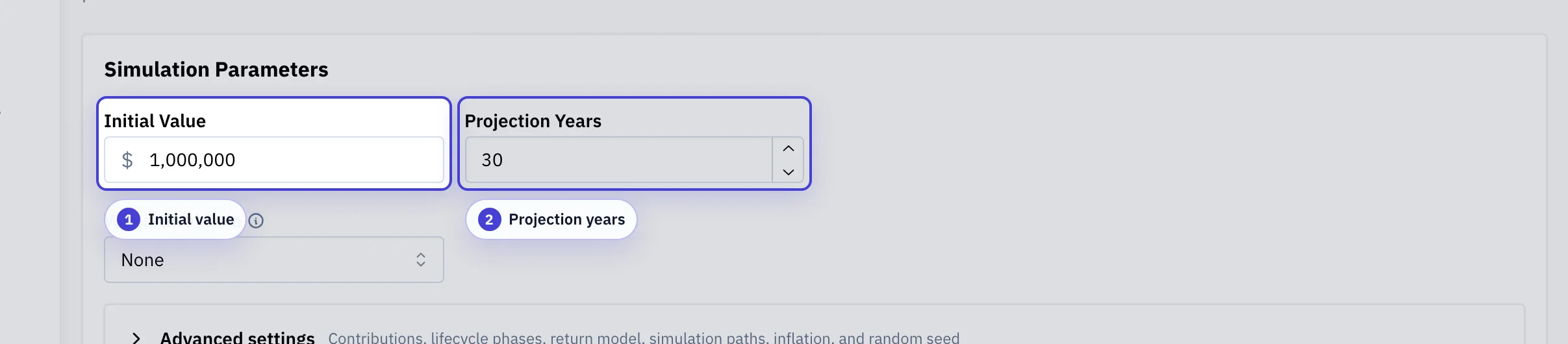
Monte Carlo configuration with initial value and projection years highlighted

Initial value: Starting portfolio balance applied to every simulated path.

Projection years: How many years each path runs. Longer horizons compound both growth and sequence risk.

Pick the spending rule

The withdrawal section decides whether the portfolio absorbs market stress, the spending level absorbs it, or both share.

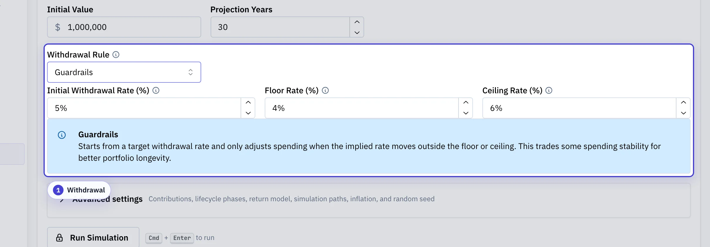
Monte Carlo withdrawal section showing the spending-rule selector and rule-specific parameters

Rule selector: Switches between fixed dollar, percent, guardrails, VPW, Guyton-Klinger, CAPE, and RMD.

Rule parameters: The inputs below the selector change to match the rule (e.g. floor/ceiling for guardrails).

Open Advanced when assumptions matter

Most paths-vs-paths comparisons require explicit return model and seed choices.

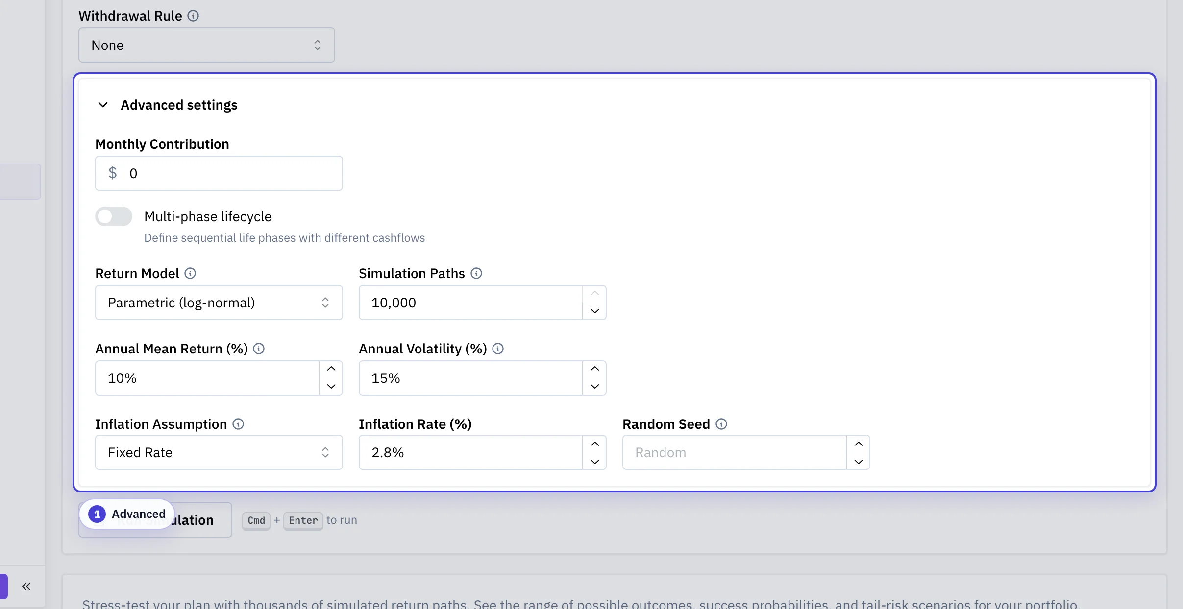
Monte Carlo advanced settings showing return model, seed, inflation, and source-portfolio controls

Return model: Parametric, historical bootstrap, block bootstrap, Student-t, or regime-switching. Each implies a different theory of how markets behave.

Random seed: Fix the seed when comparing two assumption sets so the only thing changing is the assumption itself.

Configuration	What It Means	Why It Matters
Initial value	Portfolio value at the start of the simulation.	This anchors every path and determines the dollar scale of withdrawals, contributions, and ending wealth.
Years	Number of years each simulated path runs.	Longer horizons expose the plan to more sequence risk and compounding uncertainty.
Simulations	Number of generated paths.	More paths make percentile and failure-rate estimates more stable, but they do not make the model itself more true.
Return source and model	The return generator, such as parametric assumptions, historical bootstrap, block bootstrap, Student-t, or regime switching.	Model choice controls whether paths preserve historical samples, serial patterns, fat tails, or simplified normal-like behavior.
Random seed	A fixed value used to reproduce the same random draws.	Use a seed when you need a stable comparison between two assumption sets.
Inflation model	How nominal spending and cashflows change over time.	Inflation assumptions can change real spending power and failure timing even when nominal returns are unchanged.
Withdrawal strategy	The spending rule used during each path, such as fixed dollar, percentage, guardrails, VPW, or RMD.	Spending rules change who absorbs market stress: the portfolio, the spending level, or both.

Common pitfalls

Reading the median path as a forecast

The median is the middle of a distribution, not a prediction. The 10th and 90th percentile bands matter just as much.

Comparing parametric and historical bootstrap without re-fixing the seed

Fix the random seed so the only thing changing between two runs is the assumption you actually want to test.

Cranking the path count to fight noisy results

More paths only sharpen the estimate of the same model. If results feel wrong, revisit the return model and inflation assumptions first.

Ignoring the spending path

Adaptive rules (guardrails, VPW, Guyton-Klinger) absorb market stress by adjusting spending. The terminal balance alone hides that, so read the spending-path chart.

Features

Five return models: parametric (log-normal), historical bootstrap (i.i.d.), block bootstrap, Student-t (fat-tailed), and regime-switching (2-state Markov)
Optional rolling-historical companion: replay the same plan over every overlapping past window of matching length so Monte Carlo and history can be compared side by side
Spending-rule support: fixed, percentage, guardrails, VPW, Guyton-Klinger, CAPE-based, and RMD-based
Failure-rate analysis across simulated paths
Percentile fan charts showing outcome ranges across paths
Multi-phase lifecycle plans with phase-specific cashflows and optional external income
Spending-path analysis showing how realized spending changes through time
Survival-curve analysis showing when paths begin to deplete
Representative sampled scenarios for downside, median, and upside path inspection
Library portfolio and research-asset integration with ticker modifiers

When To Use It

Estimate a range of ending wealth over a fixed horizon.
Test a withdrawal policy against many simulated paths.
Compare how inflation, spending, or return-model choices change tail outcomes.

For the exact historical behavior of a specific portfolio configuration, use Portfolio Backtest instead. See Historical Backtest vs Monte Carlo for a comparison.

Return Sources

Source	Model	What It Uses
Parametric assumptions	Parametric (Log-Normal)	Annual mean return and annual volatility entered in the form.
Historical returns	Historical Bootstrap	Resampled returns from a prior backtest or Library portfolio.
Historical blocks	Block Bootstrap	Contiguous blocks of historical returns, which preserve short serial patterns.
Student-t (fat-tailed)	Parametric, Student-t	Log returns drawn from a Student-t distribution calibrated to the historical log mean and standard deviation. Lower degrees of freedom produce fatter tails; defaults to ML-fit from history, clamped to [3, 30]. Returns the fitted dof in the response.
Regime-switching	2-state Markov	Tags each step as bull or bear based on trailing returns, then samples blocks from same-state historical runs. Transition matrix and stationary bear fraction are returned. Falls back to plain block bootstrap when only one regime is observed.

See the simulation models comparison guide for assumptions, defaults, and when to reach for each model.

Main Inputs

Initial value: starting portfolio value in dollars.
Years: simulation horizon.
Simulations: number of generated paths.
Random seed: optional seed for reproducible results.
Inflation model: whether nominal cash flows stay fixed or move with inflation assumptions.
Withdrawal strategy: the spending rule used during the run.

Withdrawal Strategies

Each strategy determines how much is withdrawn from the portfolio each period. Fixed strategies keep spending constant; adaptive strategies adjust based on portfolio performance, market conditions, or remaining time horizon.

Fixed Dollar: withdraw a constant inflation-adjusted dollar amount each year. Spending is predictable, but the portfolio bears all market risk.
Percent of Portfolio: withdraw a fixed percentage of the current portfolio value each year. Spending fluctuates with performance, but the portfolio never reaches zero.
Guardrails: start from a target withdrawal rate and inflate each year, but clamp spending when the implied rate drifts outside a floor/ceiling band. Balances income stability with portfolio protection.
Variable Percentage (VPW): withdraw a percentage that changes each year based on remaining time horizon and equity allocation. Uses an amortization formula (PMT-based) to spread the portfolio over the remaining years, drawing more as the horizon shortens.
Guyton-Klinger: start from an initial withdrawal rate and apply two path-dependent rules each year. The capital preservation rule reduces spending when the implied rate exceeds a threshold; the prosperity rule increases it when the rate falls below a threshold. Cuts and raises are percentage adjustments (typically 10%).
CAPE-Based: set annual spending as a fraction of the portfolio scaled by the inverse of the CAPE (Shiller PE) ratio, clamped to a floor and ceiling rate. Withdraws less when valuations are high and more when they are low.
RMD-Based: divide the portfolio by the IRS Uniform Lifetime Table divisor for the current age each year. Spending rises naturally as the divisor shrinks with age. For ages below 72, extrapolated divisors produce conservative (smaller) withdrawals.

What you'll see in the result

Fan chart: Percentile bands of portfolio value through time. The width of the fan is the uncertainty.
Terminal wealth distribution: Histogram of where each path ended. Median, mean, and tails are different stories.
Success rate: Share of paths that completed the horizon without depleting. Pair this with the survival curve to see when failures cluster.
Spending path: 10th, 50th, and 90th percentile spending across paths. Shows how much an adaptive rule actually adapts.
Representative scenarios: A downside, median, and upside path picked from the simulation set so you can inspect drawdown shape and depletion timing directly.

Read The Outputs

Fan chart: percentile bands of portfolio value through time.
Terminal wealth: the distribution of ending values across paths.
Success rate: share of paths that complete the horizon without reaching zero.
Tail metrics: measures focused on adverse outcomes rather than the median path.
Spending path: when withdrawals are active, the results include 10th, 50th, and 90th percentile spending paths so you can see how spending itself evolves over time, not just the ending balance. In multi-phase runs with additional income, this reflects total spending delivered rather than only the portfolio-funded portion.
Survival curve: shows the share of simulations still above zero over time, which makes depletion timing visible instead of reducing the answer to a single terminal success rate.
Safe withdrawal rate: estimated spending level that satisfies the configured confidence target when that analysis is enabled.
Representative scenarios: realized downside, median, and upside paths selected from the simulation set so you can inspect drawdown shape, depletion timing, and spending differences without relying only on percentile bands. When the analytical fast path is used, these become percentile-derived representative paths rather than sampled scenarios.
Rolling-historical companion: when enabled, the same plan is replayed across every overlapping past window of matching length. Percentile bands use the same definitions as the Monte Carlo side, so disagreements between the two reflect assumption differences rather than metric differences. Disabled by default because it roughly doubles engine cost for history-based models.

Median and average outcomes are only part of the result. The lower percentiles and failure metrics describe downside behavior.

Library Portfolios And Ticker Modifiers

When the simulation uses a Library portfolio, its historical return series becomes the input to the Monte Carlo model. If that portfolio includes ticker modifiers, the transformed return series is used automatically.

Glossary

Percentile: If you sort all simulated outcomes from worst to best, the 10th percentile is the value 10% of paths fell below. The 50th is the median.
Failure / success rate: Failure means the portfolio reached zero before the horizon ended. Success rate is one minus the failure rate.
Sequence-of-returns risk: Two plans with the same average return can end very differently if the bad years happen early in retirement. Monte Carlo surfaces this directly.
Bootstrap: Resampling actual historical returns instead of drawing from a parametric distribution. Block bootstrap preserves short serial patterns.
Survival curve: The cumulative share of paths still solvent at each point in time.
Safe withdrawal rate: The largest spending level that satisfies a configured success-rate target across the simulated paths.
VPW (Variable Percentage Withdrawal): A spending rule that amortizes the portfolio over the remaining years, withdrawing more as the horizon shortens.
RMD: Required Minimum Distribution. A spending rule based on the IRS Uniform Lifetime Table divisor for the current age.