Portfolio Optimizer
Portfolio Optimizer estimates allocations from historical data. Different modes answer different questions: one in-sample allocation, a full frontier of efficient portfolios, a walk-forward allocation process, or a Black-Litterman estimate that combines market equilibrium with explicit views.
Open Portfolio Optimizer →Use this when
Use Portfolio Optimizer to estimate weights for a given objective. For example, the highest Sharpe portfolio, or the minimum-volatility portfolio across a set of candidate assets. The result is an estimate, not a finished strategy.
Good for
- Sketching candidate weights for a small set of assets and an explicit objective.
- Tracing the efficient frontier to see how risk and return trade off.
- Combining your views with market equilibrium via Black-Litterman.
Reach for a different tool when
- Validating an allocation in detail. Hand the weights to Portfolio Backtest.
- Forecasting future returns. The optimizer estimates from history; it does not predict.
Portfolio Optimizer walkthrough
Choose the universe and optimizer mode before tuning constraints.
Treat optimizer output as an allocation estimate, not a final backtest.
Send candidate weights to Portfolio Backtest for validation with charts and saved-analysis support.
First run
Select assets
Use a small universe first so weights and constraints are easy to inspect.
Choose a mode
Mean-Variance, Efficient Frontier, Walk-Forward, Walk-Forward Validation, and Black-Litterman each answer a different question.
Set constraints
Constrain leverage, shorting, position sizes, and objective-specific limits.
Validate elsewhere
Use Portfolio Backtest before treating weights as a usable strategy.
Define the universe and optimization question
The Strategy & Assets section is where every optimizer run begins.
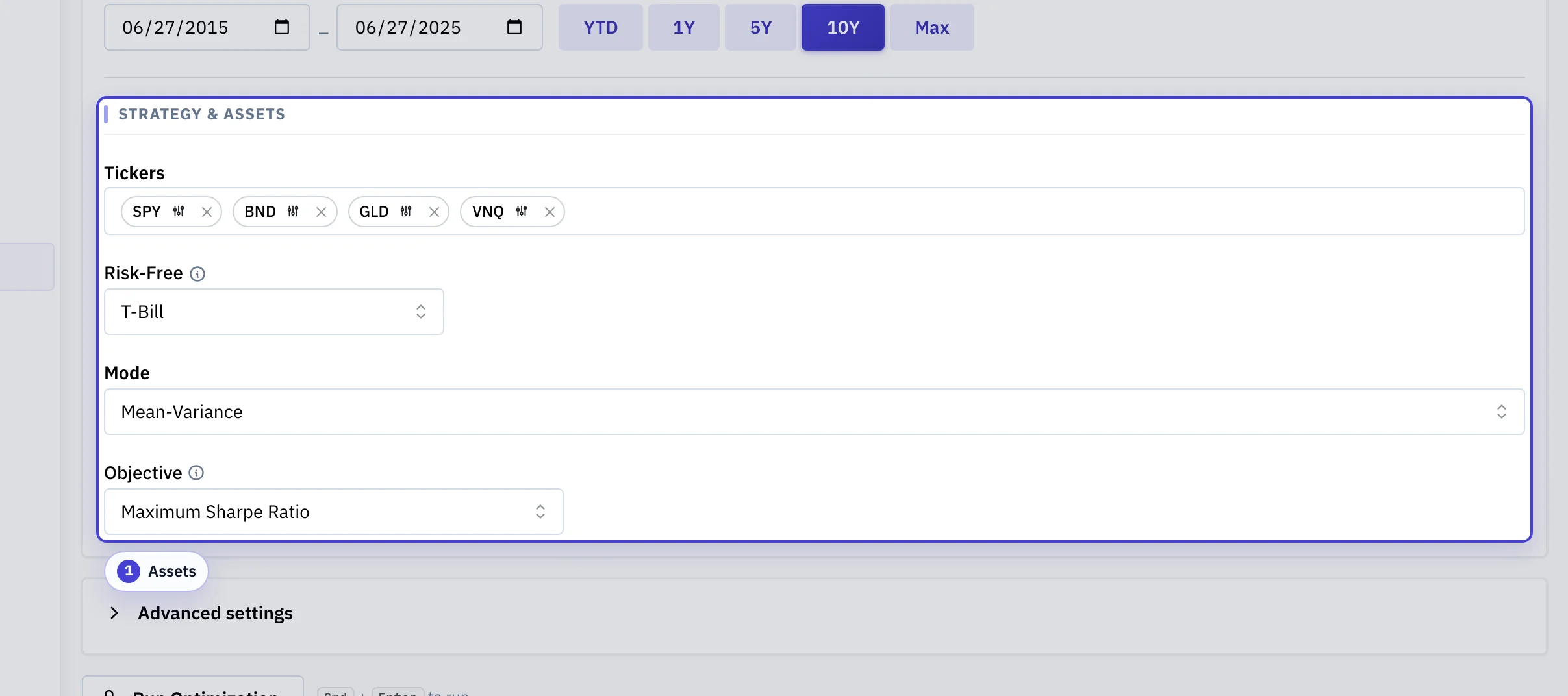
Assets: The candidate tickers the optimizer is allowed to hold, with the mode and objective controls beside them. Anything you leave out cannot appear in the result; the objective's info icon explains when to use each.
Constrain what the optimizer is allowed to pick
Constraints turn a mathematical optimum into something implementable.
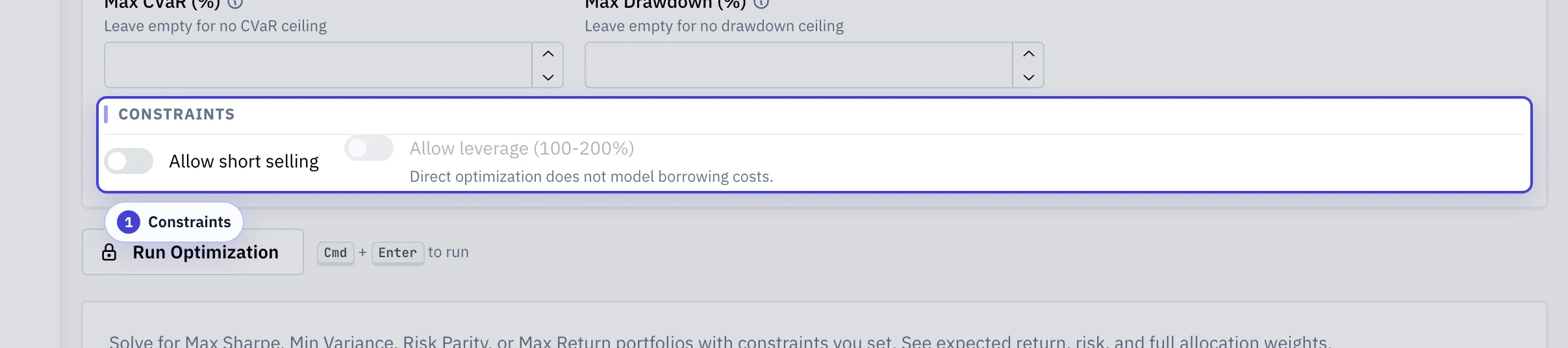
Constraints: Long-only, leverage, and per-asset weight bounds, plus optional metric bounds (minimum CAGR/Sortino, maximum volatility, CVaR, drawdown) that compose with the chosen objective.
Configuration Guide
Optimizer settings define an estimation problem. The output is a candidate allocation, not proof that the allocation will work out of sample.
| Configuration | What It Means | Why It Matters |
|---|---|---|
| Asset universe | The list of tickers the optimizer is allowed to hold. | The optimizer cannot choose assets outside the universe, so omitted candidates and redundant assets both shape the result. |
| Mode | The optimization workflow: single allocation, efficient frontier, walk-forward backtest, or Black-Litterman. | Different modes answer different questions. Do not compare weights across modes without comparing the assumptions behind them. |
| Objective | The metric the optimizer tries to improve, such as Sharpe, return, drawdown, CVaR, or another supported target. | The chosen objective determines what tradeoff the optimizer treats as success. |
| Date range | The sample used to estimate returns, risk, covariance, and walk-forward windows. | Optimizer output can be highly sample-sensitive, especially when the universe is broad or history is short. |
| Risk-free rate | The baseline return used in Sharpe, Sortino, and tangency calculations. | A higher risk-free rate can change the relative appeal of volatile assets and cash overlays. |
| Constraints | Rules such as long-only, leverage, position bounds, sector limits, turnover caps, and metric limits. | Constraints are part of the model. They can make results more implementable, but they can also hide sensitivity. |
| Walk-forward settings | Rolling window length and rebalance cadence used in optimizer backtest mode. | These settings decide what information would have been available at each historical decision point. |
Common pitfalls
Treating optimized weights as a strategy
The optimizer estimates from a single sample of history. Send the weights to Portfolio Backtest before relying on them.
Optimizing on a tiny window
Short windows produce unstable estimates and brittle weights. Span at least one major regime when you can.
Adding many similar assets and expecting diversification
Highly correlated assets distort covariance estimates. Cull near-duplicates first, then re-run.
Comparing modes side by side
Mean-Variance is one allocation; Efficient Frontier is a curve; Walk-Forward is a process. Compare the right pair to the right question.
Features
- Walk-forward backtesting with rolling optimization windows
- Black-Litterman views for incorporating investor conviction
- Full efficient frontier visualization
- Cash overlay and borrowing spread assumptions
- Constraints: sector limits, turnover caps, position bounds
- Direct metric constraints for return, volatility, tail risk, Sortino ratio, and drawdown
- Export to Portfolio Backtest for full validation
Modes
| Mode | What It Returns | What The Historical Window Means |
|---|---|---|
| Mean-Variance | One allocation optimized for the selected objective. | Used to estimate expected returns and covariance directly from the full sample. |
| Efficient Frontier | A set of efficient portfolios across the risk-return curve. | Used to estimate the same inputs as mean-variance mode. |
| Walk-Forward | Realized walk-forward metrics and the latest resulting allocation. | Split into repeated trailing windows for re-optimization. |
| Walk-Forward Validation | Train/test validation: fit on train windows, evaluate the same weights out-of-sample. | Split into one or more train/test pairs so out-of-sample results are reported separately from the fit. |
| Black-Litterman | Posterior expected returns and one resulting allocation. | Used to estimate the covariance matrix and equilibrium inputs. |
Choose The Right Optimizer Mode
| Question | Mode |
|---|---|
| What is the single best allocation for a given objective? | Mean-Variance |
| What are the efficient allocations across the risk-return curve? | Efficient Frontier |
| How would periodic re-optimization have performed historically? | Walk-Forward |
| Do these weights generalize to unseen data? | Walk-Forward Validation |
| How do explicit views change the allocation relative to market equilibrium? | Black-Litterman |
Mean-Variance and Efficient Frontier are in-sample estimates from the full date range. Backtest mode splits the window into walk-forward steps. Black-Litterman combines equilibrium with user views.
The optimizer returns an allocation estimate. Use the handoff to Portfolio Backtest when you need a full historical result with charts, tables, and saved-analysis support.
Backtest Mode Inputs
- Objective: realized walk-forward metric to optimize, such as CAGR, Sharpe, Sortino, Calmar, UPI, Omega, max drawdown, Ulcer Index, CVaR 95%, longest drawdown, SWR, or PWR.
- Rolling window: trailing history used at each re-optimization step.
- Rebalance frequency: how often the allocation is updated in the walk-forward process.
- Max holdings: upper bound on the number of included assets.
- Minimum included weight: smallest weight that may remain in the resulting allocation.
Read The Outputs
- Weights: the allocation implied by the selected mode and settings.
- Frontier points: efficient portfolios traced across the risk-return surface.
- Mode-specific metrics: such as realized walk-forward metrics in backtest mode or posterior-return details in Black-Litterman mode.
The optimizer returns an allocation estimate, not a portfolio backtest by itself. Use the handoff back into Portfolio Backtest when you want a full historical result view with charts, tables, and saved-analysis support.
Video walkthrough
Walkthrough
Video walkthrough
Optimization Objectives
In Mean-Variance mode, each objective tells the optimizer what to prioritize:
- Maximum Sharpe Ratio: finds the portfolio on the efficient frontier with the highest risk-adjusted return (excess return per unit of volatility). This is the classic tangency portfolio from modern portfolio theory.
- Minimum Volatility: finds the global minimum variance portfolio. Ignores expected returns and focuses on the lowest-variance allocation in the feasible set.
- Risk Parity: equalizes the risk contribution of each asset. Instead of targeting a specific return/risk level, it ensures every asset contributes the same amount of risk to the total portfolio.
- Maximum Diversification: maximizes the diversification ratio (weighted average standalone asset volatility divided by portfolio volatility). For uncorrelated assets this reduces to inverse-volatility weighting; in general it tilts toward low-correlation breadth without using expected-return estimates. Long-only and fully invested; short selling and leverage are not supported.
- Maximum Return: maximizes expected return subject to a volatility ceiling you specify. Set a target volatility (e.g. 15%) and the optimizer finds the highest-returning portfolio that stays at or below that risk level.
- Minimum CVaR: minimizes Conditional Value at Risk (expected shortfall) at the 95% confidence level. CVaR measures the average loss in the worst 5% of days, making it more sensitive to tail risk than volatility.
- Maximum Sortino Ratio: like maximum Sharpe, but only penalizes downside volatility. Upside volatility (prices going up more than expected) is not counted as risk.
In Backtest mode, objectives are scored on the realized walk-forward portfolio path:
| Objective | What It Prioritizes |
|---|---|
| CAGR, Sharpe, Sortino | Higher realized growth or risk-adjusted return. |
| Calmar, UPI, Omega | Higher path-aware return quality, with drawdown or gain/loss penalties. |
| Max Drawdown, Ulcer Index, CVaR 95% | Lower drawdown depth, drawdown persistence, or historical tail loss. |
| Longest Drawdown, SWR, PWR | Shorter time underwater, higher safe withdrawal rate, or higher perpetual withdrawal rate. |
The Efficient Frontier
Every time you optimize, the tool also computes the efficient frontier, the curve of all portfolios that offer the highest possible return for each level of risk. The chart shows:
- Frontier curve (indigo line): the set of optimal portfolios. Points below this curve are suboptimal (you could get more return for the same risk, or less risk for the same return).
- Max Sharpe portfolio (red star): the tangency portfolio where a line from the risk-free rate is tangent to the frontier. This point has the steepest risk-return tradeoff.
- Min Volatility portfolio (green diamond): the leftmost point on the frontier, representing the lowest-possible risk allocation.
- Individual assets (colored circles): each asset plotted at its own risk-return coordinates. These typically lie below the frontier, showing the diversification benefit of combining assets.
Hover over any point on the frontier to see the exact portfolio weights, return, volatility, and Sharpe ratio for that allocation.
Cash Overlay And Borrowing Spread
The cash overlay mode extends the efficient frontier to model explicit lending and borrowing. Instead of assuming all capital must be invested in risky assets, the frontier includes three regimes:
- Net cash (lending): when risky-asset allocation is below 100%, idle capital earns the cash rate. Portfolio volatility scales linearly with the risky allocation fraction, producing the lending segment of the capital market line.
- Fully invested: the standard Markowitz frontier where all capital is allocated to risky assets.
- Borrowing (leverage): when risky-asset allocation exceeds 100%, borrowed capital costs the cash rate plus the borrow spread. This creates the borrowing segment of the capital market line, which is flatter than the lending segment due to the higher cost of leverage.
The asymmetry between lending and borrowing rates creates a kinked capital market line rather than the single straight line in textbook models. The tangency portfolio (maximum Sharpe point) is identified on the lending segment, representing the optimal risky portfolio to combine with cash.
Each frontier point is labeled with its allocation category (net cash, fully invested, or borrowing) so you can see where your selected portfolio falls on the leverage spectrum.
Understanding The Metrics
After Mean-Variance optimization, these metrics summarize the optimal portfolio:
- Expected Return: annualized return estimated from historical daily returns (or your forward-looking inputs). Expressed as a percentage (e.g. 8.5% means the portfolio is expected to return 8.5% per year).
- CAGR: realized geometric annual growth from the historical fixed-weight path. This is the metric used when you set a minimum CAGR constraint.
- Volatility: annualized standard deviation of returns. Measures the total variability of the portfolio. A volatility of 12% means daily returns have a standard deviation of about 0.76% (12% / sqrt(252)).
- Sharpe Ratio: (return - risk-free rate) / volatility. Negative Sharpe means the portfolio underperforms the risk-free rate.
- Sortino Ratio: like Sharpe but uses only downside deviation in the denominator.
- Daily CVaR 95%: the average daily loss in the worst 5% of historical trading days. For example, a CVaR of 2.1% means that on the worst 5% of days, the portfolio lost an average of 2.1%.
- Rebalancing Bonus: the diversification return from periodic rebalancing. Positive values mean that a rebalanced portfolio would have earned a return premium over a buy-and-hold approach with the same initial weights. Larger bonuses indicate more diversification benefit.
Price Modes
- Total Return: uses adjusted prices that include dividends and distributions.
- Raw: uses unadjusted closing prices, keeping dividends and distributions separate.
Constraints
- Short selling: allows negative asset weights.
- Leverage: allows total gross exposure above 100% where the mode supports it.
- Target volatility: applies in objectives that require a risk target.
- Direct metric constraints: can require a minimum CAGR and Sortino ratio, plus maximum volatility, CVaR, and drawdown. These constraints compose; objectives such as maximum Sharpe search only among portfolios that satisfy every requested constraint.
Example: maximum Sharpe with a 10% minimum CAGR ignores portfolios below that CAGR floor, even if their Sharpe ratio is higher. If no portfolio satisfies the direct constraints, Mean-Variance mode returns an error instead of falling back to an unconstrained allocation.
Advanced Constraints (Backtest Mode)
Backtest mode supports optional metric and turnover constraints under the Advanced Constraints panel. These are checked against the final walk-forward result.
- Metric floors: require minimum values for metrics such as CAGR or Sharpe ratio. Values use the same units as the results table (percent for return and volatility metrics, raw numbers for ratios).
- Metric ceilings: require maximum values for metrics such as volatility or max drawdown.
- Per-asset bounds: set minimum and maximum weight constraints on individual assets.
- Max turnover: cap the one-way turnover per rebalance. When a rebalance would exceed the cap, the previous weights are retained for that period.
Contradictory constraints (floor exceeding ceiling on the same metric, or duplicate entries) are rejected before the optimizer runs. When no feasible portfolio satisfies all metric constraints, the response includes the best unconstrained result along with a warning identifying which constraint was violated.
Covariance Estimation
The optimizer estimates covariance as the sample covariance of the selected historical returns and enforces positive definiteness before solving.
In direct optimize mode, Advanced settings can apply linear covariance shrinkage toward a diagonal target and expected-return shrinkage toward the cross-asset arithmetic mean. Each control is an intensity in [0, 100]%: 0 is a no-op, 100 collapses to the target.
Shrinkage applies only to direct optimize. The efficient frontier, backtest, and walk-forward modes use the sample covariance on each fitting window and do not surface shrinkage controls.
Forward-Looking Parameters
The API can override historical expected returns, volatilities, and correlations with externally supplied assumptions. When those overrides are present, the optimizer uses them instead of the historical estimates.
If shrinkage is also supplied, it is applied on top of the forward-looking overrides: covariance shrinks toward its own diagonal, expected returns shrink toward the cross-asset mean of the supplied returns. Leave both shrinkage controls at zero to consume forward-looking inputs verbatim.
Black-Litterman Optimization
Black-Litterman (BL) is an alternative to classic mean-variance optimization that blends market equilibrium with your personal views. Instead of relying entirely on historical returns (which are noisy), BL starts with the returns implied by current market-cap weights (the "equilibrium") and then tilts toward your views.
Switch to BL mode using the Strategy toggle at the top of the optimizer form. The optimizer interface changes to show BL-specific inputs described below.
How it works
- Equilibrium prior: BL reverse-engineers the expected returns that would make the market-cap-weighted portfolio optimal (via π = δΣw). These "implied returns" are the starting point.
- Investor views: you overlay your own beliefs (e.g. "SPY will return 10%" or "SPY will outperform BND by 3%") with a confidence level. BL combines these views with the equilibrium using Bayesian math.
- Posterior returns: the result is a set of blended expected returns that respect both the market consensus and your views. High-confidence views tilt the posterior more; low-confidence views barely change it.
- Optimal weights: the optimizer uses these posterior returns to find the best portfolio weights. With no views, you get back the market-cap weights (a sanity check).
Inputs
- Tau (τ): uncertainty scalar on the equilibrium prior (default 0.05, range 0.01-0.5). Smaller values trust the market equilibrium more; larger values let views have more influence. A common rule of thumb is τ = 1/T where T is the number of years of data.
- Risk Aversion (δ): controls the equilibrium return magnitude (default 2.5, range 0.5-10). Higher values imply the market demands more return per unit of risk. Standard estimates for equity markets range from 2 to 4.
- Long-only constraint: when enabled (the default), all weights are constrained to [0, 1]. When disabled, the optimizer uses the analytic unconstrained solution (allowing short positions) while still requiring weights sum to 100%.
- Market-Cap Weights: the equilibrium starting point. Choose "Auto-fetch" to pull market caps from yFinance (with a fallback for ETFs/tickers without market-cap data), or "Manual" to enter custom weights that sum to 100%.
Views
Views are the core of Black-Litterman. Each view has:
- Absolute view: "Asset X will return Y% annualized." For example, "SPY returns 10%" at 80% confidence.
- Relative view: "Asset X will outperform Asset Y by Z%." For example, "SPY outperforms BND by 3%" at 70% confidence.
- Confidence (0.01-0.99): how sure you are about the view. Higher confidence tilts the posterior more. A confidence of 0.5 is a moderate belief; 0.9 is very strong conviction.
Views with incomplete fields (no asset selected or no return entered) are automatically skipped. You can have up to 20 views.
Results
The BL results panel shows three tabs:
- Weights: the optimal portfolio weights from the BL posterior.
- Returns: equilibrium vs. posterior returns for each asset, with the shift highlighted in green (positive) or red (negative).
- View Attribution: shows how each individual view independently shifts weights relative to the equilibrium. Note that these per-view effects are not additive since BL blending is non-linear.
Saved Analyses And Handoffs
Save the current optimizer run when you want to reopen the same mode, inputs, and result later. Use the resulting weights in Portfolio Backtest when you want to test that allocation in a full backtest workflow.
Limitations And Caveats
- Estimation error: optimal weights are only as reliable as the return and covariance estimates. Historical data may not represent future relationships, especially during market condition changes (e.g. rising vs. falling rate environments).
- Concentration risk: mean-variance optimization can produce extreme allocations (e.g. 90% in one asset). This is a known issue when expected return estimates are noisy. Risk parity avoids this by ignoring expected returns.
- Transaction costs: the optimizer does not account for trading costs, bid-ask spreads, or taxes. Frequent rebalancing to maintain optimal weights may erode returns in practice.
- Stationarity assumption: the optimizer assumes that return distributions are stationary (the same in the future as in the past). Correlations between assets can change significantly, especially during market crises when correlations tend to spike toward 1.0.
Glossary
Glossary
- Mean-Variance
- Optimization that trades expected return against variance (volatility squared). The classic Markowitz formulation.
- Efficient frontier
- The set of portfolios with the highest expected return for each level of risk. Anything below the frontier is dominated.
- Tangency portfolio
- The frontier portfolio with the highest Sharpe ratio given the risk-free rate. Where a line from cash is tangent to the frontier.
- Walk-forward
- Re-optimize on each trailing window, then evaluate forward. Approximates what the strategy could have done with information available at each point in time.
- Black-Litterman
- A method for combining market-implied equilibrium returns with your explicit views, weighted by your confidence.
- Covariance shrinkage
- Pulling a noisy sample covariance matrix toward a structured target to stabilize the estimate when data is limited.
- CVaR
- Conditional Value at Risk. The average loss in the worst tail (e.g. the average return in the worst 5% of cases).
- Turnover
- How much of the portfolio is traded between two rebalances. High turnover usually means more cost and more tax friction.