
Case study: the pre-tax winner that loses after tax
This case study compares a high-turnover rule-driven portfolio with a lower-turnover benchmark for a single New York resident earning $200,000.
On this page
The goal
This example compares a high-turnover strategy with a simpler portfolio in a modeled taxable account. Read after-tax ending value alongside pre-tax return.
We compare two portfolios from 2010-01-04 through 2025-12-31 with a $10,000 starting principal:
| Portfolio | Construction | Role In Comparison |
|---|---|---|
| Rule-driven tax magnet | 70% UPRO/SHY rule-driven strategy + 20% SPY + 10% AGG | High-turnover taxable portfolio under test. |
| Benchmark 80/20 | 80% SPY + 20% AGG | Lower-turnover comparison portfolio. |
Step 1: validate the predictor in Signal Analyzer
Start in Signal Analyzer. The Strategy Builder rule uses one predictor: whether SPY is above or below its 30-day simple moving average (SMA). The goal is to check whether the indicator has a measurable relationship with a later outcome before turning it into a trading rule.
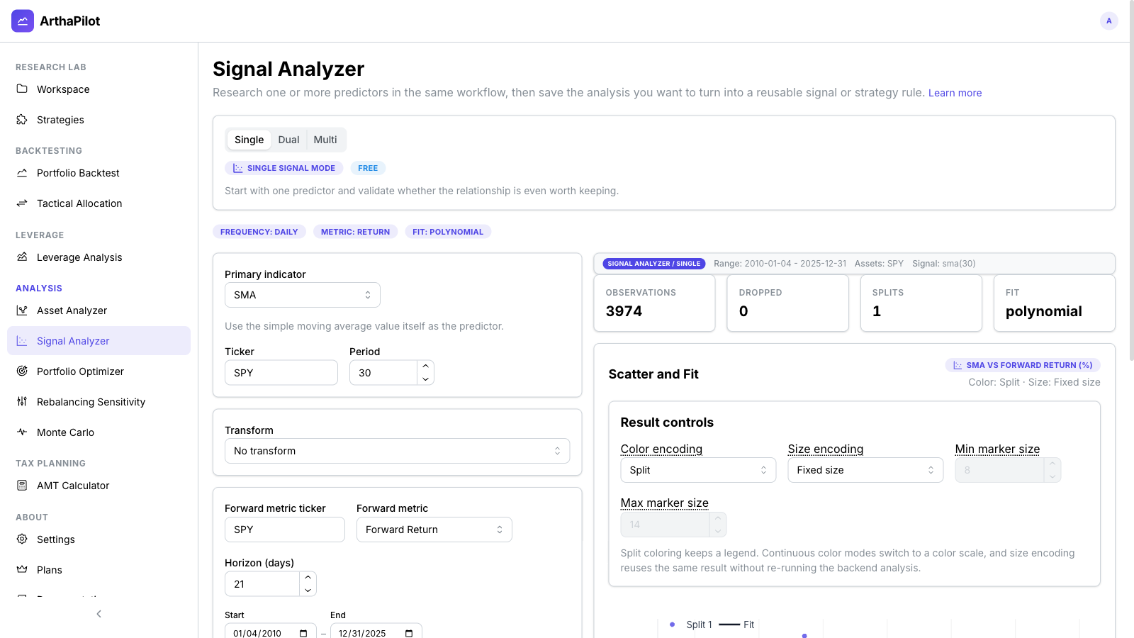
- Target: SPY forward 21-day return
- Indicator: SPY 30-day SMA
- Purpose: measure whether the signal separates forward returns before introducing leverage and turnover
Step 2: build the strategy
Use Strategy Builder to implement a two-state rule:
- Risk-On: 100% UPRO when SPY is above its 30-day simple moving average
- Risk-Off: 100% SHY as the fallback state
- Trading frequency: Daily
- Benchmark: SPY
Step 3: run the pre-tax Portfolio Backtest
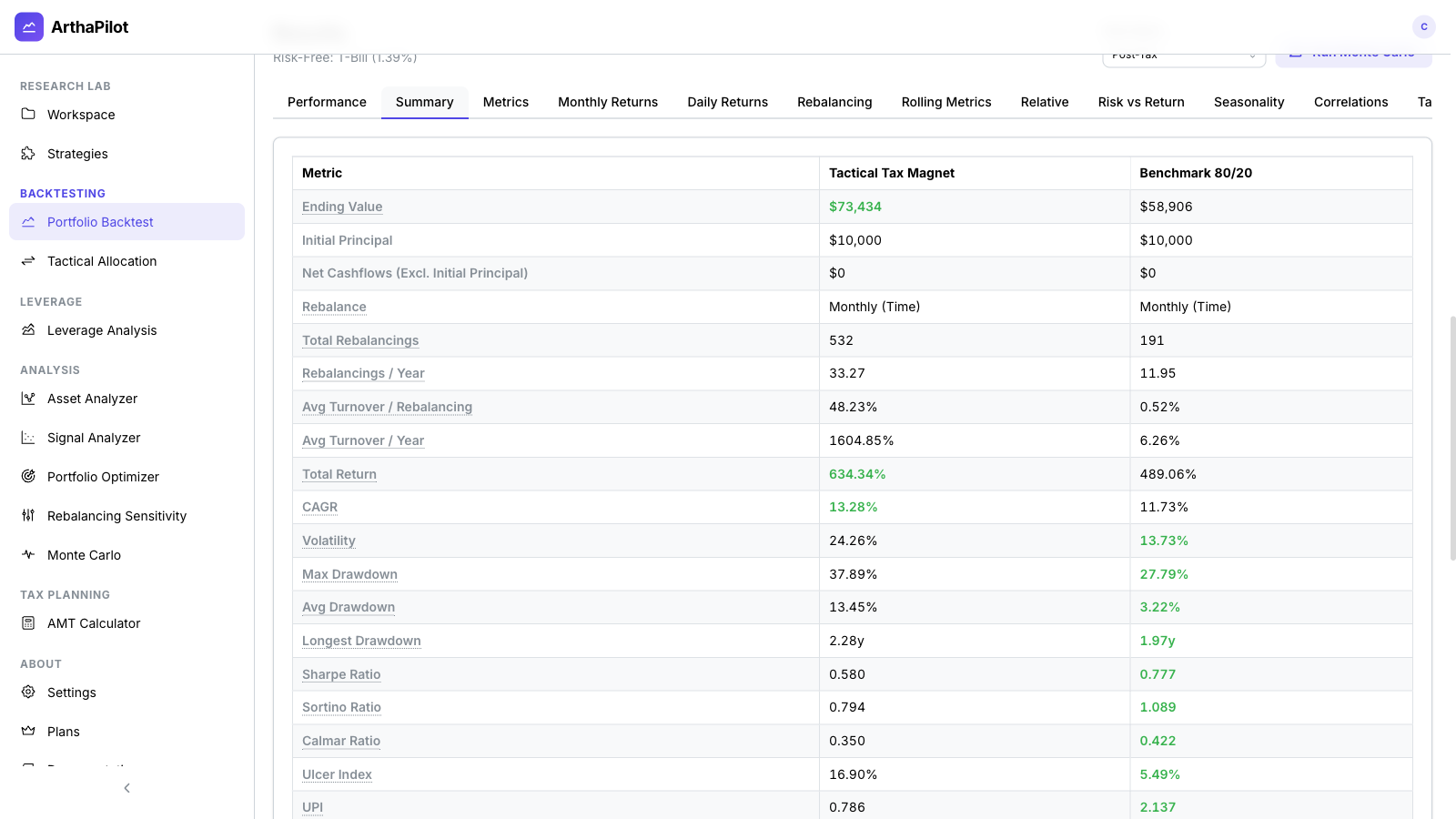
Compare this portfolio with a benchmark in Portfolio Backtest using Price Mode = Total Return and monthly portfolio rebalancing. On this first pass, the rule-driven portfolio has the higher ending value and higher CAGR.
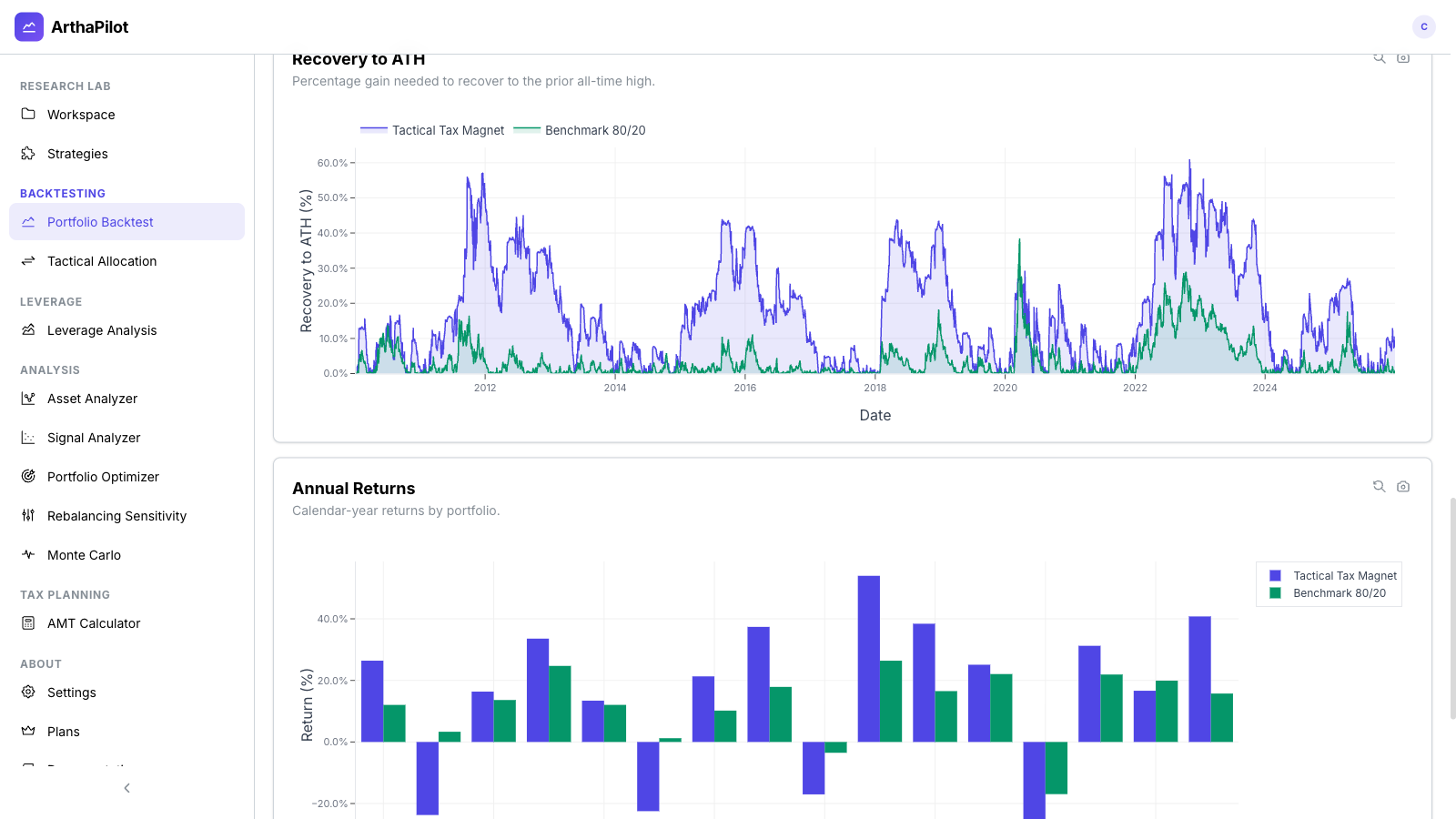
| Metric | Rule-Driven Tax Magnet | Benchmark 80/20 |
|---|---|---|
| Ending value | $73,434 | $58,906 |
| CAGR | 13.28% | 11.73% |
| Sharpe ratio | 0.580 | 0.777 |
| Max drawdown | 37.89% | 27.79% |
Step 4: turn on the tax profile
Next, enable Tax-Aware mode and model the investor:
- Filing status: single
- Annual income: $200,000
- Resident state: New York
- Lot selection: optimized
- Account type: taxable brokerage
Step 5: compare the after-tax result
The tax analysis tab plots pre-tax and after-tax value for each portfolio and summarizes the after-tax outcome:
| After-tax outcome | Rule-Driven Tax Magnet | Benchmark 80/20 |
|---|---|---|
| After-tax ending value | $31,440 | $52,585 |
| After-tax CAGR | 7.43% | 10.94% |
| Tax drag (annualized) | 7.38% | 0.80% |
| Total taxes paid | $28,626 | $3,089 |
In this run, the portfolio with the higher pre-tax ending value has about $21,000 less after tax.
Step 6: inspect the cause
The summary tables show why the ranking changes:
- The rule-driven portfolio executed 532 rebalances, versus 191 for the benchmark.
- Average turnover per year was 1604.85%, versus 6.26% for the benchmark.
- The tax summary shows $120,502 of short-term gains and $163,499 of wash-sale-disallowed losses for the rule-driven portfolio.
- The benchmark pays less tax because it trades less and realizes far fewer short-term gains.
Step 7: check Rebalancing Comparison
Use Rebalancing Comparison to see how frequencies and offsets affect the lower-turnover portfolio.
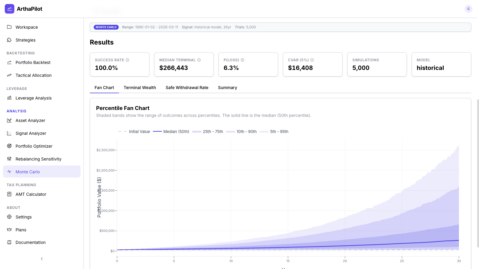
Step 8: run Monte Carlo on the surviving portfolio
Use Monte Carlo to inspect the forward distribution of the lower-turnover portfolio.
Key takeaways
In this modeled period, turnover, short-term gains, and wash-sale effects reverse the pre-tax ranking. Compare both pre-tax and after-tax results before interpreting a taxable strategy.